Likelihood Lab
This lab was written by Paul Lewis - see his Phylogenetics main page; with some tweaks by MTH
Goals
The goal of this lab exercise is to show you how to conduct maximum likelihood analyses in PAUP* and use PAUP* to see how we can use LRT to choose an appropriate model.
Getting started
You can work on this lab on your own laptop or via the cluster
If you are working on the cluster use< login to the cluster (ssh username@hpc.crc.ku.edu) and type the following command:
srun --time=02:00:00 --ntasks=1 --nodes=1 --partition=bi --pty /bin/bash -lif you have access to the BI computation queues, OR
srun --time=02:00:00 --ntasks=1 --nodes=1 --partition=eeb --pty /bin/bash -lif you want to use the EEB partition.
What to turn in
Use a text editor to answer the following questions as you work
Are chlorophyll-b taxa together in the F81 tree?
answer:

What are the empirical base frequencies for this data set?
answer:

What is the log likelihood of this tree under this "empirical base frequencies" version of the F81 model?
answer:

What proportion of sites are constant?
answer:

What are the maximum likelihood estimates (MLEs) of the base frequencies?
answer:

What is the log likelihood of this tree under the "estimated base frequencies" version of the F81 model?
answer:

What parameters are being estimated using the F81 model?
answer:

Does this model fit the data better than the "empirical base frequencies" version of the F81 model?
answer:

What is the MLE of the transition/transversion ratio under the HKY85 model?
answer:

What is the MLE of the transition/transversion _rate_ ratio under the HKY85 model?
answer:

What is the log likelihood of this tree under the HKY85 model?
answer:

What parameters are being estimated using the HKY85 model?
answer:

Does the HKY model fit the data better than the F81 model?
answer:

The transition/transversion rate ratio (kappa) is the ___ divided by the ___.
answer:

The transition/transversion ratio (tratio) is the ___ divided by the ___.
answer:

What is the MLE of pinvar under the HKY85+I model?
answer:

Is the MLE of pinvar larger or smaller than the proportion of constant sites?
answer:

Why are these two proportions different? That is, how can a site be constant but not invariable?
answer:

What is the log likelihood of this tree under the HKY85+I model?
answer:

What parameters are being estimated using the HKY85+I model?
answer:

What is the MLE of the gamma shape parameter under the HKY85+G model?
answer:

What is the log likelihood of this tree under the HKY85+G model?
answer:

What parameters are being estimated using the HKY85+G model?
answer:

What is the MLE of the gamma shape parameter under the HKY85+I+G model?
answer:

What is the MLE of the pinvar parameter under the HKY85+I+G model?
answer:

Is the MLE of the shape parameter higher or lower under the HKY85+I+G model compared to the HKY85+G model? Explain why this is so.
answer:

What is the log likelihood of this tree under the HKY85+I+G model?
answer:

What parameters are being estimated using the HKY85+I+G model?
answer:

What is the likelihood ratio test statistic for F81 vs. HKY85?
answer:

How many degrees of freedom for this test?
answer:

What is the significance (P-value) for this test?
answer:

Does allowing for a transition/transversion bias make a significant difference?
answer:

What is the likelihood ratio test statistic for a comparison of HKY+I to HKY?
answer:

What is the critical value for this likelihood ratio test (of HKY vs HKY+I)? That is, what is the smallest likelihood ratio test statistic that would be significant at the 0.05 level?
answer:

Does the HKY85+I model explain the data significantly better than an equal rates HKY85 model?
answer:

Does the HKY85+G model explain the data significantly better than an equal rates HKY85 model?
answer:

Does the HKY85+G model explain the data better than HKY85+I? Why can't you use a likelihood ratio test to compare these two models?
answer:

Does the HKY85+I+G model explain the data significantly better than either HKY85+I or HKY85+G alone?
answer:

Does the model you have selected place all the chlorophyll-b organisms together?
answer:
Download the data file algae.nex
Download the data file algae.nex using the following curl command on the cluster:
curl -Ok https://gnetum.eeb.uconn.edu/courses/phylogenetics/lab/algae.nex
Our goal for this lab will be to see if we can determine which aspects of sequence evolution are most important for getting the tree correct. The accepted phylogeny (based on much evidence besides these data) places all the chlorophyll-b-containing plastids together (Lockhart, Steel, Hendy, and Penny, 1994).
Thus, there should be a branch in the tree separating all taxa from the two that lack chlorophyll b. The 2 taxa that lack chlorophyll b are: the cyanobacterium Anacystis (which has chlorophyll a and phycobilin accessory pigments) and the chromophyte Olithodiscus (which has chlorophylls a and c).
Obtain the maximum likelihood tree under the F81 model
The first goal is to learn how to obtain maximum likelihood estimates of the parameters in several different substitution models. Use PAUP* to answer the following questions. Start by obtaining the maximum likelihood tree under the F81 model.
Launch paup in the same directory as the algae.nex file using:
./paup4a168_centos64 or
./paup if you renamed paup
Start a log file and execute the data file:
log start file=lab3log.txt ;
execute algae.nex ;
Tell PAUP to use likelihood and the F81 model for a heuristic search:
paup> set criterion=likelihood;
lset nst=1 basefreq=empirical;
hsearch;
The nst=1 tells PAUP* that we want a model having just one substitution rate parameter (the JC69 and F81 models both fall in this category). The basefreq=empirical tells PAUP* that we want to use simple estimates of the base frequencies. The empirical frequency of the base G, for example, is the value you would get if you simply counted up all the Gs in your entire data matrix and divided by the total number of nucleotides. The empirical frequencies are not usually the same as the maximum likelihood estimates (MLEs) of the base frequencies, but they are quick to calculate and often very close to the corresponding MLEs.
Issue the following command to show the tree:
showtrees;
One problem is that the tree is drawn in such a way that it appears to be rooted within the flowering plants (tobacco and rice). Specifying the cyanobacterium Anacystis as the outgroup makes more sense biologically:
outgroup Anacystis_nidulans;
showtrees;
If you want to see the edge lengths drawn proportionally to the estimate of their length (in the expected number of substitutions per site) use:
describe 1 / plot=phylogram;
Are chlorophyll-b taxa together in the F81 tree?
Save this tree to a file named f81.tre using the savetrees command:
savetrees file=f81.tre brlens;
If you ever need to read this tree back in, use the gettrees command:
gettrees file=f81.tre;
Now get PAUP* to show you the maximum likelihood estimates for the parameters of the F81 model used in this analysis (the 1 here refers to tree 1 in memory):
lscores 1;
cstatuscommand will give you this information)
Estimate base frequencies
Now estimate the base frequencies on this tree with maximum likelihood by adding the following 3 lines to your paup block just above the quit command (you can replace the [add new commands here] comment). Note how the lscores command is used to force PAUP* to recompute the likelihood (under the revised model) and spit out the parameter estimates.
lset basefreq=estimate;
lscores 1;
Note: the new lset command will reset the previous one (which specified basefreq=empirical). This will allow you to see the difference in likelihood when using empirical vs estimated base frequencies. The first lscores 1 command will use empirical frequencies and the second lscores 1 command will use estimated frequencies.
Estimate transition/transversion bias
Switch to the HKY85 model now and estimate the transition/transversion ratio along with the base frequencies. The way you specify the HKY model in PAUP* is to tell it you want a model with 2 substitution rate parameters (nst=2), and that you want to estimate the base frequencies (basefreq=estimate) and the transition/transversion ratio (tratio=estimated).
lset nst=2 basefreq=estimate tratio=estimate;
lscores 1;
_______divided by the_______.
_______divided by the_______.
Estimate the proportion of invariable sites
Now ask PAUP* to estimate pinvar, the proportion of invariable sites, using the command lset pinvar=estimate followed by an lscore command. The HKY85 model with among-site rate heterogeneity modeled using the two-category invariable sites approach is called the HKY85+I model.
Estimate the heterogeneity in rates among sites
Now set pinvar=0 and tell PAUP* to use the discrete gamma distribution with 5 rate categories. Here are the commands for doing this all in one step:
lset pinvar=0 rates=gamma ncat=5 shape=estimate;
lscores 1;
The HKY85 model with among-site rate heterogeneity modeled using the discrete gamma approach is called the HKY85+G model.
Estimate both pinvar and the gamma shape parameter
Now ask PAUP* to estimate both pinvar and the gamma shape parameter simultaneously (the HKY85+I+G model).
Likelihood ratio tests
In this section, you will perform some simple likelihood ratio tests to decide which of the models used in the previous section does the best job of explaining the data while keeping the number of parameters used to a minimum.
Determining significance
A model having k parameters can always attain a higher likelihood than any model having fewer than k parameters that is nested within it (you should be able to explain why this is true). The question we need to ask is: Does the more complex (i.e. more parameter-rich) models fit significantly better than simpler nested models?
To do this we will assume that the likelihood ratio test statistic LR (equal to twice the difference in log-likelihoods) has the same distribution as a chi-squared random variable with degrees of freedom (d.f.) equal to the difference in the number of estimated parameters in the two models. (A parameter whose value is fixed or which can be determined from the values of other parameters doesn’t count as an estimated parameter.)
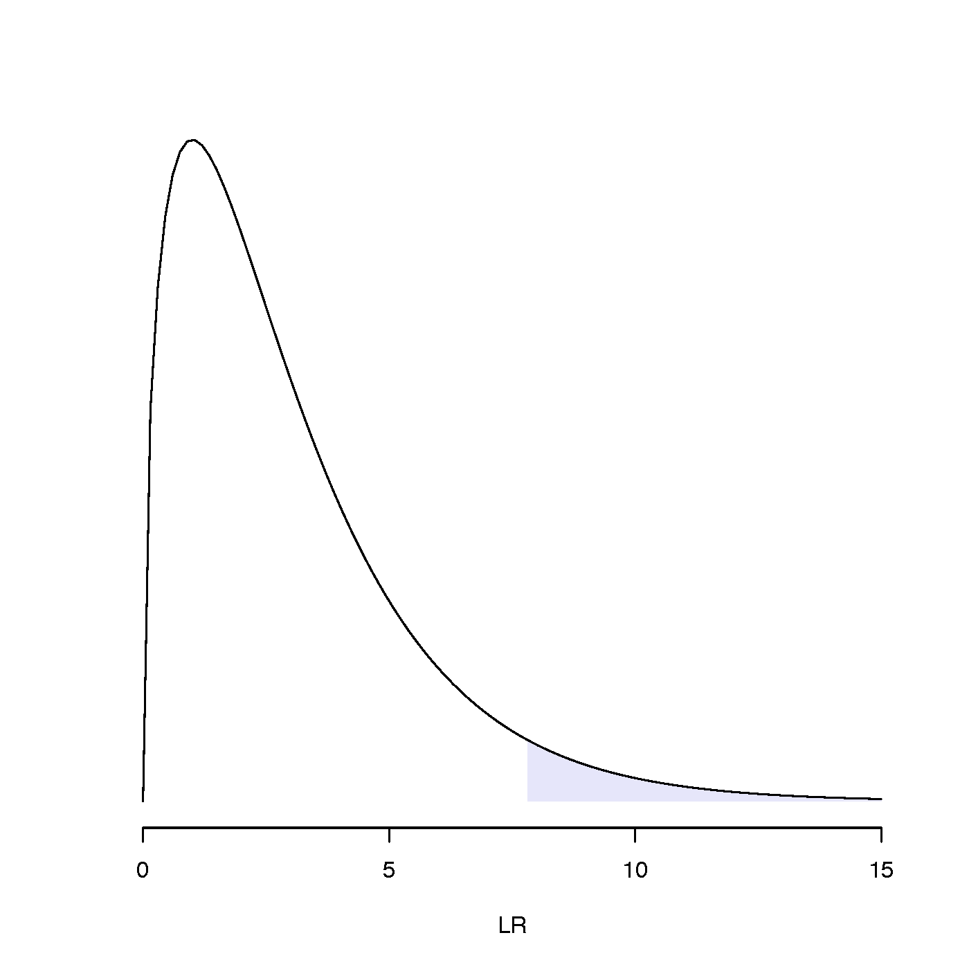
To be specific, we would like to know whether LR falls inside the 5% right tail of the chi-squared distribution (see figure to the right for an example). If it does, then it should be considered an unusually large value of LR; i.e. not a LR value that would normally arise (i.e. falls within the interval that accounts for 95% of the probability distribution) if the models were equivalent explanations of the data.
In R, you can use a command like pchisq(6.91, df=1, lower.tail=FALSE) to find that the P-value associated with a chi-squared test statistic of 6.91 is 0.008571499. Alternatively, you can look up a chi-squared table of critical values using the internet.
What parameters make the fit of the model significantly better?
The model with which we will begin is the F81 model with estimated base frequencies. Compare this F81 model to the HKY85 model, which differs from the F81 model only in the fact that it allows transitions and transversions to occur at different rates.
To calculate the likelihood ratio test statistic LR, subtract the log-likelihood of the less complex model from that of the more complex model and multiply by 2. This will give you a positive number. If you ever get a negative LR statistic, it means you have the models in the wrong order.
You should have all the numbers you need to perform these likelihood ratio tests. If, however, you have not written some of them down, and thus need to redo some of these analyses, you might need to know how to turn off rate heterogeneity using the following command:
lset rates=equal pinvar=0;
Repeat search under a better model
Earlier in the lab, you found that the F81 model with empirical base frequencies did not produce the expected tree separating chlorophyll-b organisms from the two (Anacystis and Olithodiscus) that lack chlorophyll-b. Would a new search under a better model have the same result?
Using the simplest model that you can defend (of the five we have examined: F81, HKY85, HKY85+I, HKY85+G, HKY85+I+G), perform a heuristic search under the maximum likelihood criterion. Use the template below, but make changes necessary to match the model you have chosen to use.
The next two paragraphs provide some explanation of the commands used in the template.
To make the analysis go faster, we will ask PAUP* to not re-estimate all the model parameters for every tree it examines during the search. To do this, first use the lset command to set up the model you are planning to use (be sure to specify estimate for all relevant parameters: base frequencies, shape, tratio, etc.). Use the lscores command to force PAUP* to re-estimate all of the parameters of your selected model on some tree (the tree just needs to be something reasonable, such as a NJ tree or the F81 tree you have been using).
Now, re-issue the lset command but, for every parameter that you estimated, change the word estimate to previous. After executing this new lset command, start a search using just hsearch. PAUP* will fix the parameters at the previous values (i.e. the estimates you just forced it to calculate) and use these same values for every tree examined during the search.
Template Supposing you decided that HKY85+I+G was the best model, here are the paup commands:
lset nst=2 basefreq=estimate tratio=estimate rates=gamma shape=estimate pinvar=estimate;
nj;
lscores 1;

lset nst=2 basefreq=previous tratio=previous rates=gamma shape=previous pinvar=previous;

hsearch;

showtrees;
describe 1 / plot=phylogram;
savetrees file=hky85ig.tre brlens replace;
This lab is already a bit long, so we will not take time to do it now, but I hope you realize that you could figure out exactly what parameter(s) are needed in the model to get this tree right. JC69 doesn’t do it, nor does F81 (as you may have noticed), but it actually doesn’t take much beyond JC69 to do the trick.
Literature Cited
Lockhart, P. J., Steel, M. A., Hendy, M. D., & Penny, D. 1994. Recovering evolutionary trees under a more realistic model of sequence evolution. Molecular Biology and Evolution 11(4):605–612.